Segmentation

Last reviewed: 2026-07-07.

Segmentation is the most detailed image task: instead of a box, it labels every pixel, outlining the exact shape of objects or regions. It matters in African work wherever a precise area or boundary is the point, such as measuring the exact extent of a crop field, delineating a lesion in a medical scan, or mapping land cover from satellite imagery.

What the data looks like

A segmentation dataset pairs images with pixel-level masks. Semantic segmentation labels every pixel by class without separating individual objects, while instance segmentation also tells apart one object from another of the same class. The data is dominated by the same high-value African domains, with crop-field boundary sets like LacunaLabels and land-cover sets like LandCoverNet built because precise African-landscape masks did not exist. Satellite segmentation carries its own difficulty, cloud cover, which leaves gaps that are often filled by combining optical with radar imagery.

A mask is usually stored as a PNG the same size as the image, where each pixel value is a class id, paired with a small mapping from id to class name:

field_0007.jpg          # the image
field_0007_mask.png     # same width and height; pixel value = class id

# class mapping (e.g. classes.json)
{"0": "background", "1": "crop_field", "2": "water", "3": "built_up"}

Storing the mask as a single-channel id map, rather than a colour image, keeps it exact: a colour PNG can be re-compressed and shift a pixel's value, which silently changes its class, while an id map stays faithful to what the annotator drew.

Annotation and evaluation

Pixel-level annotation is the most expensive labelling in this playbook, so design it to be feasible: use tools with smart boundary assistance, define exactly how to treat ambiguous edges and mixed pixels, and pilot to measure how long a mask really takes before committing a budget. Because masks are so detailed, agreement is best measured by overlap rather than exact match. Segmentation is evaluated with mean Intersection over Union (mIoU), and with the Dice coefficient or pixel accuracy, all of which compare predicted masks to reference masks by how much they overlap rather than demanding identical pixels.

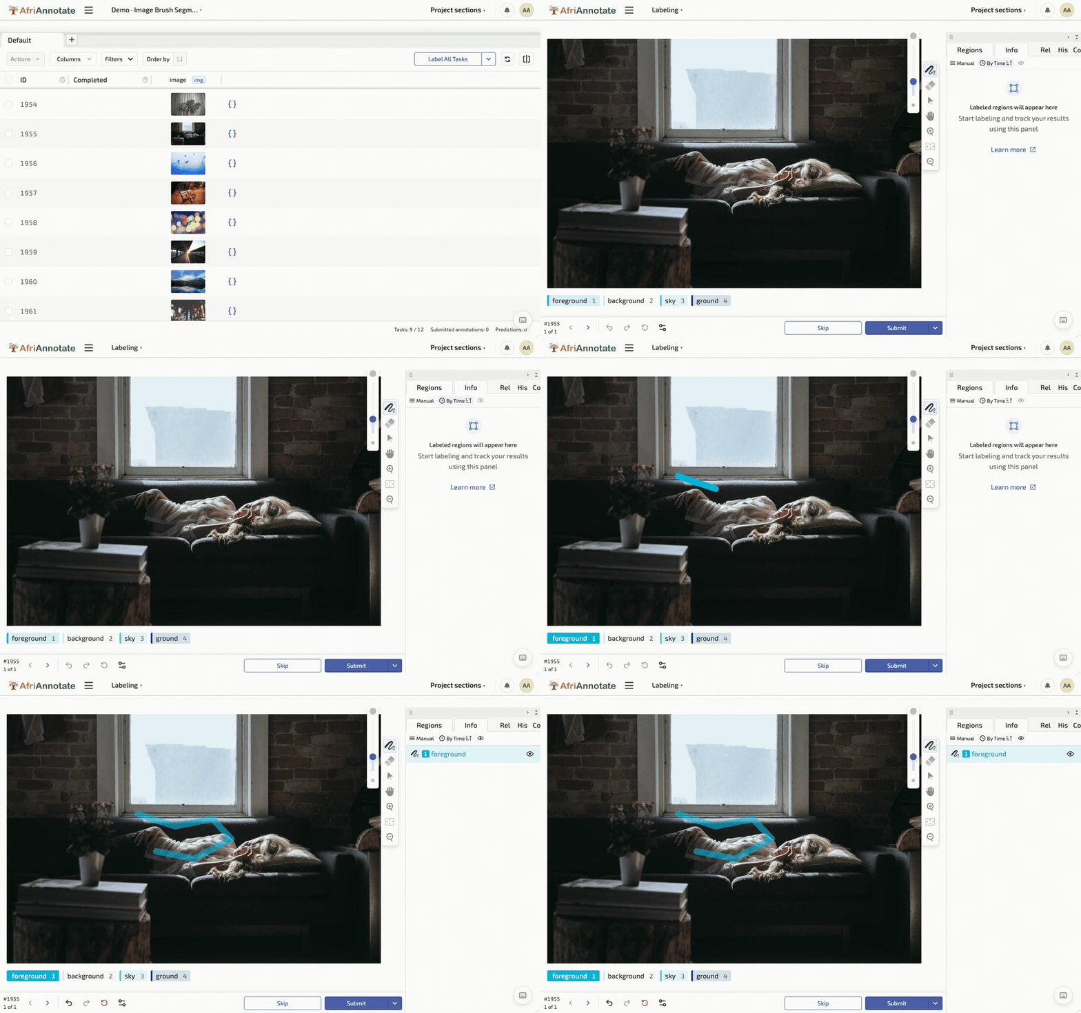
The labeling config gives the annotator a brush to paint each class onto the image:

<View>
  <Image name="image" value="$image"/>
  <BrushLabels name="mask" toName="image">
    <Label value="Crop field" background="#1F5B3F"/>
    <Label value="Water"      background="#13A4B4"/>
    <Label value="Built-up"   background="#C66A3D"/>
  </BrushLabels>
</View>

Both metrics are short to compute directly from the id-map masks, and computing them per class is what keeps a small but important region honest:

import numpy as np

def per_class_iou(pred: np.ndarray, true: np.ndarray, class_id: int) -> float:
    p, t = (pred == class_id), (true == class_id)
    union = (p | t).sum()
    return (p & t).sum() / union if union else float("nan")

def per_class_dice(pred: np.ndarray, true: np.ndarray, class_id: int) -> float:
    p, t = (pred == class_id), (true == class_id)
    denom = p.sum() + t.sum()
    return 2 * (p & t).sum() / denom if denom else float("nan")

classes = {1: "crop_field", 2: "water", 3: "built_up"}
ious = {name: per_class_iou(pred_mask, true_mask, cid)
        for cid, name in classes.items()}
print("per-class IoU:", {k: round(v, 3) for k, v in ious.items()})
print("mIoU:", round(np.nanmean(list(ious.values())), 3))

Averaging IoU across classes rather than across pixels is the deliberate choice: a thin feature like a river covers few pixels, so a pixel-weighted score would let a model ignore it entirely while still looking accurate, whereas per-class mIoU makes that failure visible.

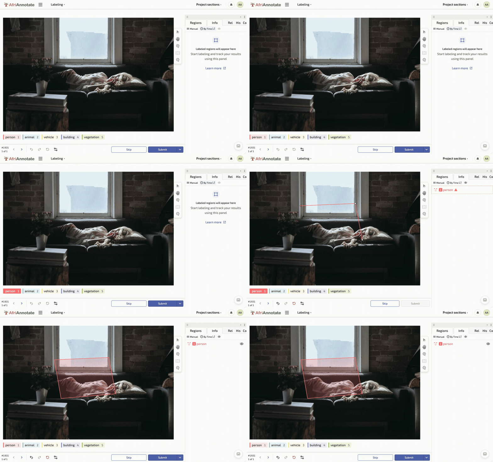
Tracing a polygon and painting a brush mask in AfriAnnotate:

Tracing a polygon in AfriAnnotate

Painting a brush mask in AfriAnnotate

The 2026 modelling landscape

Segmentation in 2026 is split between purpose-built segmentation models, foundation segmenters that generalise across tasks with minimal fine-tuning, and geospatial-domain-specific models. The workable open-model references:

Segment Anything Model (SAM 2) (Meta, 2024): the reference open foundation segmenter, Apache-2.0 licensed, promptable via boxes / points / text. Substantially reduces the cost of segmentation annotation (SAM-assisted labelling with human correction is 5-10x faster than pure manual labelling). The workable frontier for annotation-time productivity.
Mask2Former (Meta, 2021): the unified transformer-based architecture for semantic, instance, and panoptic segmentation. Fine-tuning on 500-3,000 target-domain masks produces a competitive task-specific segmenter.
OneFormer (2022) and Mask DINO (2022): competing unified segmenters; measure against Mask2Former on your specific task.
DINOv3 (Meta, 2025) as a segmentation backbone: the strongest current self-supervised pretraining for dense prediction; fine-tune a segmentation head on top for tasks with limited labelled data.
Geospatial models. Prithvi (IBM/NASA, 2023-2024) and SatMAE (2022) are the workable open geospatial foundation models for satellite-imagery segmentation (crop mapping, land cover, deforestation). Fine-tune on 500-2,000 target-region satellite tiles.
nnU-Net v2: the reference medical-imaging segmenter (CT / MRI / X-ray); still the workable default for medical-imaging African contexts.

Editorial opinion. For a new African-context segmentation project (agriculture crop-field boundaries, environment land-cover, medical-imaging lesion delineation), the shortest defensible path is: use SAM 2 to generate initial masks and human-correct them (5-10x annotation speedup), fine-tune Mask2Former or DINOv3 with a segmentation head on the corrected corpus, and report per-class IoU alongside mIoU. For satellite imagery, fine-tune Prithvi or SatMAE on target-region tiles before fine-tuning a general segmenter. The geospatial-pretrained backbones handle the multi-spectral, low-resolution, cloud-affected input distribution substantially better than general-imagery backbones.

What it will actually cost you

Segmentation is the most expensive vision annotation in the playbook. SAM 2-assisted labelling has reduced this cost substantially since 2024, but it is still 5-20x more expensive per-record than classification. Rough order-of-magnitude:

Fine-tuning Mask2Former or DINOv3 on an existing segmentation corpus. Two to four person-weeks; forty to two hundred GPU-hours.
Building a new segmentation corpus with SAM 2-assisted labelling (500-3,000 images, 5-30 classes). Six to twelve months elapsed; five to twelve person-months. Boundary adjudication is the constraint; pilot to measure per-mask time before committing.
Pure-manual segmentation labelling (where SAM 2 does not work: historical imagery, degraded scans, unusual modalities). 3-8x slower than SAM 2-assisted; budget accordingly.
Satellite-imagery segmentation with Prithvi or SatMAE fine-tuning. Three to eight months for 500-2,000 labelled tiles.
Medical-imaging segmentation with nnU-Net v2. Six to fifteen months for a domain-specific corpus (clinical labels, ethical review, patient consent).
Evaluation-only segmentation sets (200-500 masks). Two to four months; two to five person-months.
Human evaluation of segmentation output. One to two person-weeks per evaluator per 200 masks. The overlap is visually obvious in most cases; ambiguous boundaries take longer.

Known limitations to watch for

Per-class IoU is the honest number. A model that scores mIoU 0.75 overall may score 0.90 on the dominant background class and 0.30 on the small-but-important target class. The per-class breakdown is what shows failure.
Boundary annotation is inherently subjective. Two annotators mask a lesion boundary 2-5 pixels apart; two annotators mask a crop-field boundary 3-8 pixels apart. Report boundary-agreement IoU as a floor.
Class imbalance in pixel space. Rivers, roads, and thin linear features cover few pixels but matter for downstream tasks. Pixel-weighted accuracy hides this failure; per-class mIoU exposes it.
Cloud cover in satellite imagery. Optical satellite imagery is unusable under clouds. Radar imagery (Sentinel-1) fills the gap but requires multi-modal fusion, which is architecturally more complex than optical-only segmentation.
SAM 2 fails on unusual modalities. SAM 2 is trained on natural imagery. It works on general photos, degrades on medical imaging, and fails on satellite imagery at typical spectral bands. Do not assume the annotation speedup applies universally.
Mask storage as PNG must be single-channel. Colour-map PNGs re-compress and drift; single-channel id-map PNGs stay faithful. Enforce this in the export pipeline.
Instance vs. semantic segmentation are different tasks. Semantic (paint every crop-field pixel green) is cheaper than instance (paint each crop field a separately-numbered green). If downstream needs counting, plan for instance segmentation.
Consent for medical-imaging patients. Segmentation masks derived from patient scans carry the same consent obligations as the scans themselves. The data governance chapter covers the discipline.